 Quantum information technology
Complete quantum-optical process tomography
Quantum information technology
Complete quantum-optical process tomography
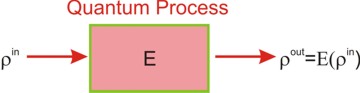 Suppose we are given a quantum "black box" that converts any quantum state ρin into some other state ρout. The purpose of quantum process tomography (QPT) is to characterize this black box in such a way that we could predict the output state for any known input. To accomplish this, we send a number of "probe" states into the black box and determine the output. Knowing the effect of the black box on the probe states, we can calculate its effect on any other state.
What should the set of probe states be? Contrary to what we've studied in undergraduate quantum mechanics, not every quantum process can be written as a linear operator. The expression
process(|ψ1> + |ψ2>) = process(|ψ1>) + process(|ψ2>)
does not always hold. For example the process of decoherence may preserve energy eigenstates |ψ1> and |ψ2> but convert their superposition (|ψ1> + |ψ2>) into an incoherent mixture
|ψ1><ψ1| + |ψ2><ψ2|. However, fortunately all quantum processes are linear with respect to density matrices:
process(ρ1 + ρ2) = process(ρ1) + process(ρ2).
This follows from the probabilistic nature of the density matrix.
Based on this linearity, we can choose the set of probe states to be the basis {ρi} in the space of density matrices. Indeed, if we can express any density matrix as a linear combination
ρinput = Σi ρi,
and measure the state process(ρi) for every ρi, then we can calculate the process output for ρinput as
process(ρinput) = Σi process(ρi).
This is one of the most common approaches to QPT.
QPT is a difficult experimental procedure. If we are dealing with an N-dimensional Hilbert space, the set {ρi}of probe states will contain N2 elements. For each element, we need to perform full quantum tomography of the process output state, i.e. determine the density matrix consisting of N2 parameters. This means that full quantum process tomography means determining N4 numbers. For example, a process on two qubits (N = 4) requires acquiring 256 large data sets! All this is in addition to the task of constructing the set of probe states experimentally, which is also challenging. This is why quantum process tomography has so far been limited to Hilbert spaces of very low dimension.
Our technique is based on the fact that coherent states form an approximate basis in the space of optical density matrices. Indeed, any optical state ρin can be written as
 ,
,
where Pρin is the state's Glauber-Sudarshan P-function [1-2] (one of the achievements for which the 2005 Nobel Prize in Physics was awarded) and |α> is the coherent state of amplitude α.
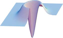
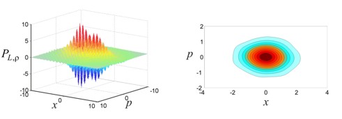 It is known that the P-function is ill-behaved: sometimes it is defined only as a generalized function. Fortunately, as shown by Klauder [3], any state can be arbitrarily well approximated by a state with a regular P-function. the figure on the left shows an example: the highly irregular P-function of the squeezed vacuum state (right panel), can be well approximated with a regular P-function (left panel).
Or procedure of studying an unknown quantum "black box" runs as follows. First, we send many different coherent states |α> into the "black box" and characterize, by means of homodyne tomography, the corresponding output states process(|α><α|). Of course, this cannot be done for all coherent states. However, we can make our measurement for as many coherent states as are necessary to confidently interpolate to the rest of the phase space. Then we can calculate the process output for any other state ρin according to 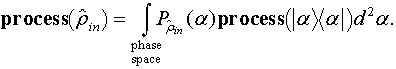
As an example we applied this protocol to a simple process that consisted of amplitude and phase modulation by means of an electro-optical modulator followed by a polarizer. We tested the reliability of the protocol by prediction the output of the process to a squeezed vacuum input. The fidelity between experimental and predicted output was greater the 99%.
More details about this work can be found in M. Lobino et al., Science 322, 563 (2008)
References